鸢尾花数据集(Iris
Dataset)是机器学习中最经典的入门数据集之一。
鸢尾花数据集包含了三种鸢尾花(Setosa、Versicolor、Virginica)每种花的
4 个特征:花萼长度、花萼宽度、花瓣长度和花瓣宽度。
接下来我们的任务是基于这些特征来预测鸢尾花的种类。
本章节案例将涵盖数据加载、可视化、特征选择、数据预处理、建立分类模型、模型评估及优化等步骤。
1、数据加载与可视化
数据加载
首先,加载鸢尾花数据集,scikit-learn 提供了直接加载鸢尾花数据集的接口。
实例
from sklearn.datasets import load_irisimport pandas as pd# 加载鸢尾花数据集 = load_iris( ) # 转换为 DataFrame 方便查看 = pd.DataFrame ( data.data , columns= data.feature_names ) [ 'target' ] = data.target [ 'species' ] = df[ 'target' ] .apply ( lambda x: data.target_names [ x] ) # 查看前几行数据 print ( df.head ( ) )
输出结果:
sepal length ( cm ) sepal width ( cm ) petal length ( cm ) petal width ( cm ) target species
0 5.1 3.5 1.4 0.2 0 setosa
1 4.9 3.0 1.4 0.2 0 setosa
2 4.7 3.2 1.3 0.2 0 setosa
3 4.6 3.1 1.5 0.2 0 setosa
4 5.0 3.6 1.4 0.2 0 setosa
此时,数据已经成功加载,并且我们可以看到每条数据的特征和对应的花卉种类。
数据可视化
为了更好地理解数据,可以通过可视化的方式查看不同特征之间的关系,我们可以使用
matplotlib 和 seaborn 库来进行可视化。
实例
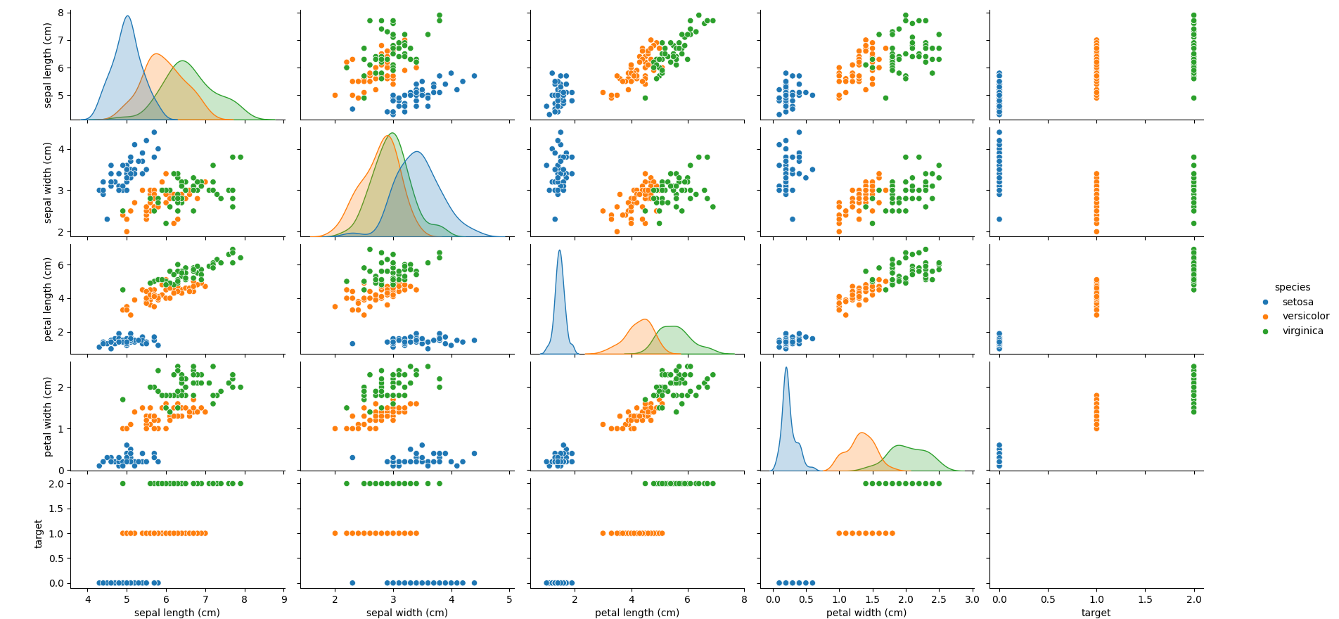
from sklearn.datasets import load_irisimport pandas as pdimport seaborn as snsimport matplotlib.pyplot as plt# 加载鸢尾花数据集 = load_iris( ) # 转换为 DataFrame 方便查看 = pd.DataFrame ( data.data , columns= data.feature_names ) [ 'target' ] = data.target [ 'species' ] = df[ 'target' ] .apply ( lambda x: data.target_names [ x] ) # 绘制特征之间的关系 pairplot ( df, hue= "species" ) show ( )
pairplot 会绘制特征之间的散点图矩阵,使用不同颜色标识不同的鸢尾花种类,这有助于我们了解各特征的分布和它们之间的关系。
显示图如下:
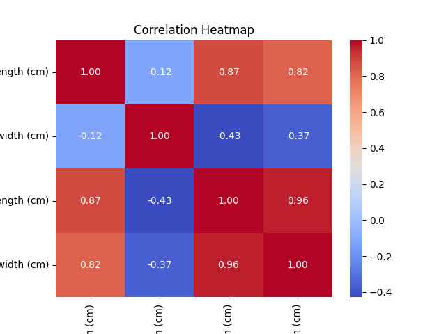
热力图可视化特征之间的相关性
通过热力图可以查看特征之间的相关性,较强的相关性可以帮助我们在建模时做出更好的选择。
实例
from sklearn.datasets import load_irisimport pandas as pdimport seaborn as snsimport matplotlib.pyplot as plt# 加载鸢尾花数据集 = load_iris( ) # 转换为 DataFrame 方便查看 = pd.DataFrame ( data.data , columns= data.feature_names ) [ 'target' ] = data.target [ 'species' ] = df[ 'target' ] .apply ( lambda x: data.target_names [ x] ) # 绘制特征之间的关系 = df.drop ( columns= [ 'target' , 'species' ] ) .corr ( ) heatmap ( correlation_matrix, annot= True , cmap= "coolwarm" , fmt= ".2f" ) title ( "Correlation Heatmap" ) show ( )
显示图如下:
2、特征选择与数据预处理
数据预处理
在机器学习中,数据预处理是非常重要的一步。
对于鸢尾花数据集,特征值已经是数值型数据,不需要太多的预处理。但是,我们可以对数据进行标准化,以提高模型的训练效果。
实例
from sklearn.preprocessing import StandardScaler# 提取特征和标签 = df.drop ( columns= [ 'target' , 'species' ] ) = df[ 'target' ] # 标准化特征 = StandardScaler( ) = scaler.fit_transform ( X)
标准化的目的是使每个特征的均值为 0,方差为 1,这对于一些基于距离的模型(如 KNN、SVM)非常重要。
特征选择
虽然鸢尾花数据集的特征比较简单,但在实际问题中,有时我们需要通过特征选择来减少特征维度,提升模型效果。
我们可以使用 SelectKBest 或 Recursive Feature Elimination
(RFE) 等方法。
例如,使用 SelectKBest 选择与标签最相关的 2 个特征:
实例
from sklearn.feature_selection import SelectKBest, f_classif# 使用卡方检验选择 2 个最相关的特征 = SelectKBest( f_classif, k= 2 ) = selector.fit_transform ( X_scaled, y) # 打印选择的特征 = selector.get_support ( indices= True ) print ( "Selected features:" , X.columns [ selected_features] )
这将选出与目标标签相关性最高的 2 个特征。
3、建立一个分类模型:使用决策树或 SVM 进行分类
使用决策树分类器
我们将首先尝试使用决策树(Decision Tree)模型进行分类。
实例
from sklearn.model_selection import train_test_splitfrom sklearn.tree import DecisionTreeClassifierfrom sklearn.metrics import accuracy_score# 划分数据集 , X_test, y_train, y_test = train_test_split( X_scaled, y, test_size= 0.2 , random_state= 42 ) # 初始化决策树分类器 = DecisionTreeClassifier( random_state= 42 ) # 训练模型 fit ( X_train, y_train) # 预测 = model_dt.predict ( X_test) # 评估模型 = accuracy_score( y_test, y_pred_dt) print ( f"Decision Tree Accuracy: {accuracy_dt:.4f}" )
使用支持向量机(SVM)进行分类
接下来,我们可以尝试使用支持向量机(SVM)进行分类。
实例
from sklearn.svm import SVC# 初始化 SVM 分类器 = SVC( kernel= 'linear' , random_state= 42 ) # 训练模型 fit ( X_train, y_train) # 预测 = model_svm.predict ( X_test) # 评估模型 = accuracy_score( y_test, y_pred_svm) print ( f"SVM Accuracy: {accuracy_svm:.4f}" )
4、评估模型并优化
模型评估
除了准确率外,我们还可以使用其他评估指标,如混淆矩阵、精度、召回率和
F1 分数等。
实例
from sklearn.metrics import classification_report, confusion_matrix# 混淆矩阵 = confusion_matrix( y_test, y_pred_dt) print ( "Confusion Matrix (Decision Tree):" ) print ( cm) # 精度、召回率、F1 分数 = classification_report( y_test, y_pred_dt) print ( "Classification Report (Decision Tree):" ) print ( report)
网格搜索调优
为了优化模型,我们可以使用网格搜索(GridSearchCV)对模型的超参数进行调优,找到最佳的参数组合。
实例
from sklearn.model_selection import GridSearchCV# 定义决策树的参数网格 = { 'max_depth' : [ 3 , 5 , 10 , None ] , 'min_samples_split' : [ 2 , 5 , 10 ] , 'min_samples_leaf' : [ 1 , 2 , 4 ] } # 初始化 GridSearchCV = GridSearchCV( estimator= DecisionTreeClassifier( random_state= 42 ) , param_grid= param_grid, cv= 5 ) # 训练网格搜索 fit ( X_train, y_train) # 获取最佳参数和最佳模型 print ( "Best Parameters:" , grid_search.best_params_ ) = grid_search.best_estimator_ # 预测和评估 = best_model.predict ( X_test) = accuracy_score( y_test, y_pred_optimized) print ( f"Optimized Decision Tree Accuracy: {accuracy_optimized:.4f}" )
通过网格搜索,我们可以找到最适合当前数据的决策树参数,并提升模型的预测准确率。
交叉验证
为了进一步评估模型的稳定性,我们可以使用交叉验证来评估模型的性能。
实例
from sklearn.model_selection import cross_val_score# 进行 5 折交叉验证 = cross_val_score( best_model, X_scaled, y, cv= 5 ) print ( f"Cross-validation Scores: {cross_val_scores}" ) print ( f"Mean CV Accuracy: {cross_val_scores.mean():.4f}" )
交叉验证可以帮助我们评估模型在不同数据子集上的表现,避免模型过拟合。
5、完整代码
以下是一个完整的代码案例,涵盖了鸢尾花数据集的加载、数据预处理、特征选择、建立分类模型、模型评估与优化等步骤。我们将使用决策树和
SVM 分类器,并通过网格搜索优化模型超参数。
实例
# 导入必要的库 import numpy as npimport pandas as pdimport seaborn as snsimport matplotlib.pyplot as pltfrom sklearn.datasets import load_irisfrom sklearn.model_selection import train_test_split, GridSearchCV, cross_val_scorefrom sklearn.preprocessing import StandardScalerfrom sklearn.tree import DecisionTreeClassifierfrom sklearn.svm import SVCfrom sklearn.metrics import accuracy_score, classification_report, confusion_matrix# 1. 数据加载 # 加载鸢尾花数据集 = load_iris( ) # 转换为 DataFrame 方便查看 = pd.DataFrame ( data.data , columns= data.feature_names ) [ 'target' ] = data.target [ 'species' ] = df[ 'target' ] .apply ( lambda x: data.target_names [ x] ) # 查看前几行数据 print ( "数据预览:" ) print ( df.head ( ) ) # 2. 数据可视化 # 绘制特征之间的关系 pairplot ( df, hue= "species" ) show ( ) # 绘制热力图查看特征之间的相关性 = df.drop ( columns= [ 'target' , 'species' ] ) .corr ( ) heatmap ( correlation_matrix, annot= True , cmap= "coolwarm" , fmt= ".2f" ) title ( "Correlation Heatmap" ) show ( ) # 3. 特征选择与数据预处理 # 提取特征和标签 = df.drop ( columns= [ 'target' , 'species' ] ) = df[ 'target' ] # 数据标准化 = StandardScaler( ) = scaler.fit_transform ( X) # 4. 建立分类模型 # 划分数据集 , X_test, y_train, y_test = train_test_split( X_scaled, y, test_size= 0.2 , random_state= 42 ) # 使用决策树分类器 = DecisionTreeClassifier( random_state= 42 ) fit ( X_train, y_train) # 预测 = model_dt.predict ( X_test) # 输出决策树的准确率 = accuracy_score( y_test, y_pred_dt) print ( f"Decision Tree Accuracy: {accuracy_dt:.4f}" ) # 使用支持向量机(SVM)分类器 = SVC( kernel= 'linear' , random_state= 42 ) fit ( X_train, y_train) # 预测 = model_svm.predict ( X_test) # 输出SVM的准确率 = accuracy_score( y_test, y_pred_svm) print ( f"SVM Accuracy: {accuracy_svm:.4f}" ) # 5. 模型评估 # 决策树模型评估 print ( "\n Decision Tree Classification Report:" ) print ( classification_report( y_test, y_pred_dt) ) print ( "\n Decision Tree Confusion Matrix:" ) print ( confusion_matrix( y_test, y_pred_dt) ) # SVM模型评估 print ( "\n SVM Classification Report:" ) print ( classification_report( y_test, y_pred_svm) ) print ( "\n SVM Confusion Matrix:" ) print ( confusion_matrix( y_test, y_pred_svm) ) # 6. 网格搜索调优 # 定义决策树的参数网格 = { 'max_depth' : [ 3 , 5 , 10 , None ] , 'min_samples_split' : [ 2 , 5 , 10 ] , 'min_samples_leaf' : [ 1 , 2 , 4 ] } # 初始化 GridSearchCV = GridSearchCV( estimator= DecisionTreeClassifier( random_state= 42 ) , param_grid= param_grid, cv= 5 ) fit ( X_train, y_train) # 获取最佳参数和最佳模型 print ( "\n Best Parameters from GridSearchCV (Decision Tree):" ) print ( grid_search.best_params_ ) # 使用最佳模型进行预测 = grid_search.best_estimator_ = best_model.predict ( X_test) # 输出优化后的决策树准确率 = accuracy_score( y_test, y_pred_optimized) print ( f"Optimized Decision Tree Accuracy: {accuracy_optimized:.4f}" ) # 7. 交叉验证 # 进行 5 折交叉验证 = cross_val_score( best_model, X_scaled, y, cv= 5 ) print ( "\n Cross-validation Scores (Optimized Decision Tree):" ) print ( cross_val_scores) print ( f"Mean CV Accuracy: {cross_val_scores.mean():.4f}" )
代码解析:
数据加载 :
1.使用 load_iris() 加载鸢尾花数据集,并将数据转换为 DataFrame
格式,以便查看和分析。
数据可视化 :1.使用 seaborn 的 pairplot 绘制各特征之间的散点图矩阵,并通过 heatmap
绘制特征之间的相关性热力图。
特征选择与数据预处理 :1.提取特征(X)和标签(y),并对特征数据进行标准化处理,使得每个特征的均值为 0,方差为
1。
建立分类模型 :1.使用 DecisionTreeClassifier 和 SVC 分别训练决策树分类器和支持向量机分类器,并评估它们在测试集上的准确率。
模型评估 :1.使用 classification_report 和 confusion_matrix
输出模型的详细评估指标,包括精度、召回率、F1 分数以及混淆矩阵。
网格搜索调优 :1.使用 GridSearchCV 对决策树模型进行超参数调优,寻找最佳的超参数组合,并输出优化后的模型准确率。
交叉验证 :1.使用 cross_val_score 进行 5 折交叉验证,评估优化后的决策树模型的稳定性和表现。
输出如下:
数据预览:
sepal length ( cm ) sepal width ( cm ) petal length ( cm ) petal width ( cm ) target species
0 5.1 3.5 1.4 0.2 0 setosa
1 4.9 3.0 1.4 0.2 0 setosa
2 4.7 3.2 1.3 0.2 0 setosa
3 4.6 3.1 1.5 0.2 0 setosa
4 5.0 3.6 1.4 0.2 0 setosa
Decision Tree Accuracy : 1.0000
SVM Accuracy : 1.0000
Decision Tree Classification Report :
precision recall f1 - score support
0 1.00 1.00 1.00 9
1 1.00 1.00 1.00 8
2 1.00 1.00 1.00 8
accuracy 1.00 25
macro avg 1.00 1.00 1.00 25
weighted avg 1.00 1.00 1.00 25
Decision Tree Confusion Matrix :
[[ 9 0 0 ]
[ 0 8 0 ]
[ 0 0 8 ]]
SVM Classification Report :
precision recall f1 - score support
0 1.00 1.00 1.00 9
1 1.00 1.00 1.00 8
2 1.00 1.00 1.00 8
accuracy 1.00 25
macro avg 1.00 1.00 1.00 25
weighted avg 1.00 1.00 1.00 25
SVM Confusion Matrix :
[[ 9 0 0 ]
[ 0 8 0 ]
[ 0 0 8 ]]
Best Parameters from GridSearchCV ( Decision Tree ):
{ 'max_depth' : 5 , 'min_samples_leaf' : 1 , 'min_samples_split' : 2 }
Optimized Decision Tree Accuracy : 1.0000
Cross - validation Scores ( Optimized Decision Tree ):
[ 1. 1. 1. 1. 1. ]
Mean CV Accuracy : 1.0000