| 蔡氏电路仿真实验
模拟电路运行
采用MATLAB进行模拟。本电路为一常微分方程的初值问题。
1.取定参数
2.matlab代码实现
3.首次模拟的图像 对比 对比
4.参数调整后,模拟的图像 对比 对比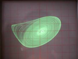
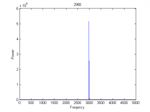
5.分析频谱
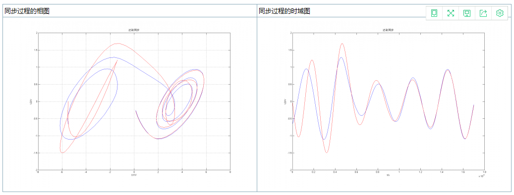
6.模拟非线性电路同步
7.非线性电路同步瞬态过程

取定参数
模拟实验中的电感电容都采用测量值,为了方便,取为定值。
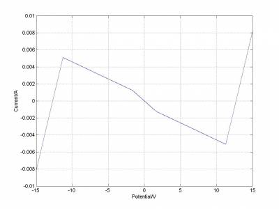
非线性负阻的I-V特性取成奇对称,数值和测量值稍作对称性修正。
代码实现
这里使用Matlab中ode45,四阶龙格库塔法求解常微分方程初值问题。C和C++的代码
I-V函数 myfun.m
function
fun=myfun(x)
if x<0
fun=-myfun(-x);
elseif x<1.664849891
fun=x*(-7.44316E-04)-5.065E-06;
elseif x<11.29059205
fun=x*(-4.003E-04)-5.778E-04;
else
fun=x*3.574E-03-4.545E-02;
end |
微分方程组 myode.m
function
dy=myode(t,y)
global gg;
dy = zeros(3,1);
G=1/gg;
C1=9.91E-9;
C2=98.2E-9;
L=23E-3;
dy=[(G*(y(2)-y(1))-myfun(y(1)))/C1;
(G*(y(1)-y(2))+y(3))/C2;
-y(2)/L];
end |
调节1/G输出图像nonlinear.m
clear;
global gg;
for gg=1800:1:2200
fs=100000;
[T,Y]=ode45('myode',0:1/fs:0.2,[0;0;0]);
X=Y(10002:end,1);
plot(Y(10002:end,1),Y(10002:end,2));
grid on
axis([-13 13 -3 3]);
xlabel('U1/V');
ylabel('U2/V');
str=[num2str(gg) '.jpg'];
saveas(gcf,str);
end |
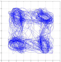
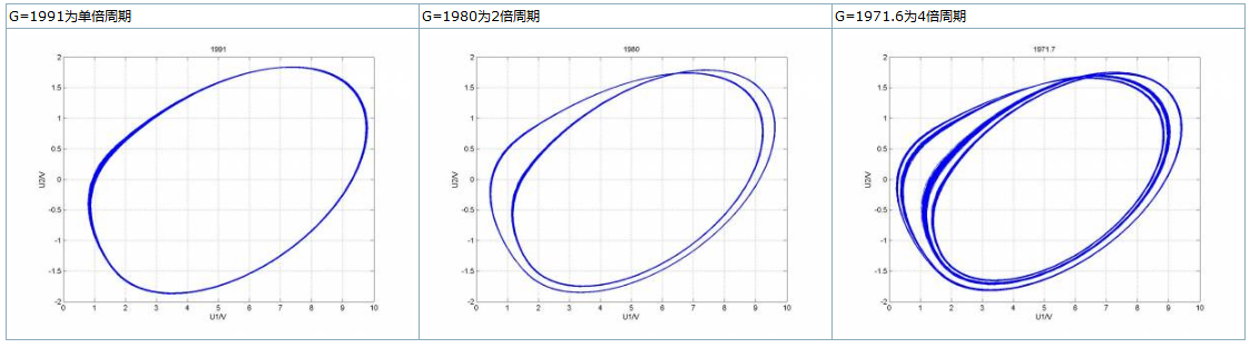
首次模拟的结果
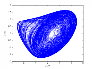
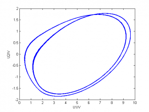
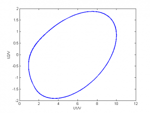
改变1/G的由小到大数值,作出U2-U1相图,可以观察到一下几种典型图样

图形变化的规律和真实实验观察到的基本一致,但是图像对应的1/G和形状与真实实验不太一致,究其原因,是我的L,C1,C2测量不准确。
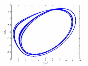
参数调整后,模拟的结果
将L、C1、C2换为参考值,再次计算。1/G在1530到2040之间变化。
C1=10E-9;
C2=100E-9;
L=18E-3; |

改变参数以后图形和实验更相似,但是变化的规律不变
分岔图分析
分岔图可以直观得看到分岔,这里用U1的最小值来画分岔图,代码如下:
clear;
fs=100000;
for gg=1992:-0.1:1940;
[T,Y]=ode23(@myode,0:1/fs:0.2,[0;0;0]);
data=Y(:,1);
n=length(data);
N=n-round(n/4);
for i=N:n-2
if data(i)<data(i-1) && data(i)<data(i+1)
&& data(i)<data(i-2) &&
data(i)<data(i+2);
plot(gg,data(i));
hold on;
else
end
end
end
beep |
分岔图:
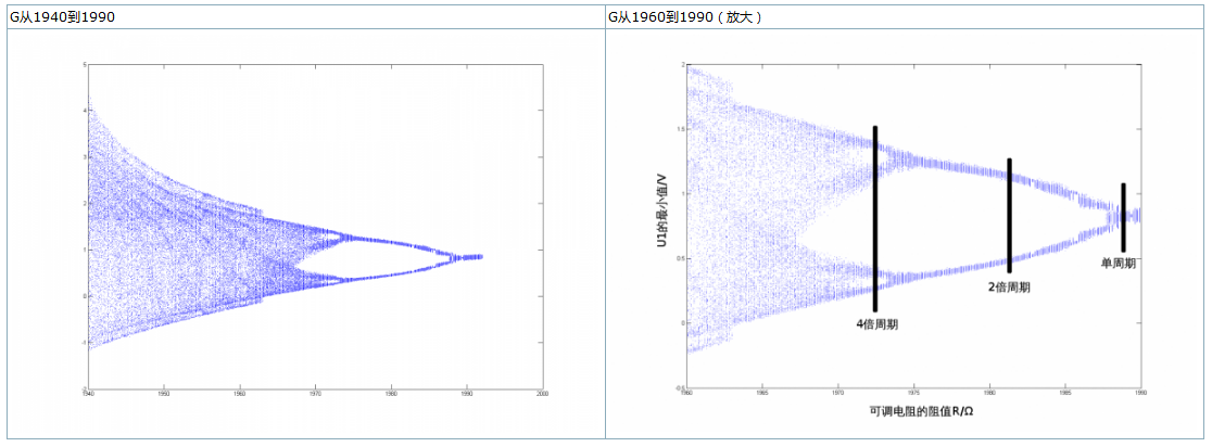
介于matlab提供的龙格库塔法函数精度很难控制,且计算缓慢,建议使用C语言进行数值计算,并提高精度。

从左边大范围的分岔图上已经清晰显示了1→2→4→8→6→5→3的分岔过程。我们将分岔图区域放大后(如右图),我们发现分岔图具有自相似性,即分形的最大特点。
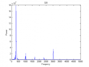
处理与分析
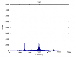
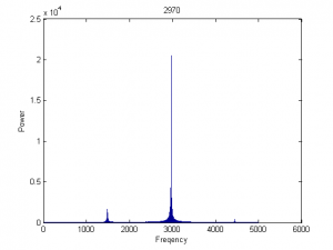
利用快速傅立叶变换分析频谱
X=fft(X);
N=length(X);
X(1) = [];
power = abs(X(1:N/2)).^2;
[mp,index] = max(power);
nyquist = 1/2;
freq = (1:N/2)/(N/2)*nyquist*fs;
figure(1);
subplot(211);
plot(freq,power), grid on
title (freq(index))
xlabel('Freqency');
ylabel('Power');
period = 1./freq;
figure(1);
subplot(212);
plot(period,power), grid on
title (period(index))
ylabel('Power');
xlabel('Period'); |
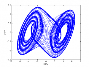
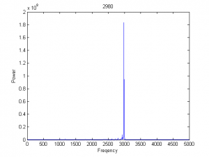
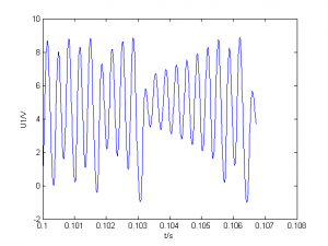
G=1500、1827、1946、1999采样
| G | 相图 | 功率谱 | 最大周期20倍时长时域图 | 说明 |
| 1500 |
 |
 |
 |
|
| 1827 |
 |
 |
 |
功率谱有5个峰,而吸引子有5层圈。最大峰位的频率与其它相比显著小 |
| 1946 |
 |
 |
 |
|
| 1971.7 |
 |
 |
 |
|
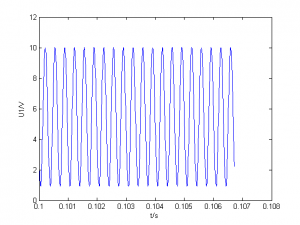
| 1980 |
 |
 |
 |
|
| 1999 |
 |
 |
 |
|
模拟非线性电路同步
随机产生两个混沌电路的初始参数,只需要改变如下一行。
| [T,M]=ode45(@myode,0:1/fs:0.19,[rand();rand();rand()/1000]); |

非线性电路同步的瞬态过程
在极短时间内两个电路达到了同步
2016 nonlinear circuit with python implementation
Claim: This is a brief documentation of using
python to understand the simulation of the Nonlinear
circuit problem.
Background: Compared with Matlab , python is weigh
more powerful in handling object-oriented simulation
despite of simulink.
Also,python is really a hot languange which will
be beneficial for our scientific computing.
这里面要求环境装上scipy和numpy,一般windows用pip,而OS用户就可以用brew,linux的话大家都懂
import
numpy as np
from scipy.integrate import odeint
import matplotlib.pyplot as plt
def Nlfunction(V_1):
Ga=-0.00076
Gb=-0.00049
E=15.0
retg=Gb*V_1+(Gb-Ga)/2*(abs(V_1-E)-abs(V_1+E))
return retg
def delta(y,t):
global R
C1=9.91e-9
C2=98.2e-9
l=23e-3
G=1/R
ret_delta =np.array([(G*(y[1]-y[0])-Nlfunction(y[0]))/C1,
(G*(y[0]-y[1])+y[2])/C2,
-y[1]/l])
return ret_delta
time=np.linspace(0,0.2,10000)
r=range(1930,1960,1)
yinit=np.array([0.0,0.0,0.1])
global R
for R in r:
y = odeint(delta,yinit,time)
plt.figure()
plt.plot(y[1000:,0],y[1000:,1])
plt.xlabel('U_1')
plt.ylabel('U_2')
plt.legend()
plt.savefig('%domega'%R)
plt.clf() |
张贴一些相图
R=1800

R=1841

R=1859

|