|
时间序列
在一个时间段中不同时刻得到的数据,一般有的是固定频率(比如每小时)。这里要介绍的内容主要包括三部分:
1.Timestamps, specific instants
in time
2.Fixed periods, such as the
August of 2014
3.Intervals of time, indicated
by a start and end timestamp
用到的工具主要就是 Pandas 了。
相关工具
和时间相关的几个modules主要有 datetime, time 和 calendar
In
[317]: from datetime import datetime
In [318]: now = datetime.now()
In [319]: now
Out[319]: datetime.datetime(2012, 8, 4, 17,
9, 21, 832092)
In [320]: now.year, now.month, now.day
Out[320]: (2012, 8, 4) |
datetime objects 和 string 之间的转换
datetime
objects转string
In [9]: stamp = datetime(2011, 1, 3)
In [10]: str(stamp) 或者 stamp.strftime('%Y-%m-
%d')
Out[10]: '2011-01- 03' |
string
转 datetime
In [332]: value = '2011-01-03'
In [333]: datetime.strptime(value, '%Y-%m-%d')
Out[333]: datetime.datetime(2011, 1, 3, 0,
0)
In [334]: datestrs = ['7/6/2011', '8/6/2011']
In [335]: [datetime.strptime(x, '%m/%d/%Y')
for x in datestrs]
Out[335]: [datetime.datetime(2011, 7, 6, 0,
0), datetime.datetime(2011, 8, 6, 0, 0)] |
还可以调用parser.parse来自动解析时间
In
[336]: from dateutil.parser import parse
In [337]: parse('2011-01-03')
Out[337]: datetime.datetime(2011, 1, 3, 0,
0)
dateutil 可以解析绝大多是时间的表达式
>In [338]: parse('Jan 31, 1997 10:45 PM')
Out[338]: datetime.datetime(1997, 1, 31,
22, 45)
国际上,一般先写日子再写月份
In [339]: parse('6/12/2011', dayfirst=True)
Out[339]: datetime.datetime(2011, 12, 6,
0, 0) |
Pandas的应用
Pandas 是设计用来处理 arrays of dates的,作为DataFrame当中的axis
index或者 column.
to_datetime 方法用于解析许多不同类别的日期表达式。
In
[340]: datestrs
Out[340]: ['7/6/2011', '8/6/2011']
In [341]: pd.to_datetime(datestrs)
Out[341]:
<class 'pandas.tseries.index.DatetimeIndex'>
[2011-07-06 00:00:00, 2011-08-06 00:00:00]
Length: 2, Freq: None, Timezone: None |
to_datetime 还可以处理 the values that should be considered
missing (None, empty string, etc.):
In
[342]: idx = pd.to_datetime(datestrs + [None])
In [343]: idx
Out[343]:
<class 'pandas.tseries.index.DatetimeIndex'>
[2011-07-06 00:00:00, ..., NaT]
Length: 3, Freq: None, Timezone: None
In [344]: idx[2] #最后加上去的[None]
Out[344]: NaT
In [345]: pd.isnull(idx)
Out[345]: array([False, False, True], dtype=bool)
NaT (Not a Time) is pandas’s NA value for
timestamp data. |
Series 基础
在pandas中最基本的时间序列文件是 a Series indexed by timestamps
In
[346]: from datetime import datetime , from
pandas import *
In [347]: dates = [datetime(2011, 1, 2), datetime(2011,
1, 5), datetime(2011, 1, 7),datetime(2011,
1, 8), datetime(2011, 1, 10), datetime(2011,
1, 12)]
In [348]: ts = Series(np.random.randn(6),
index=dates)
In [349]: ts
Out[349]: # 以时间作为index,一列是6位的随机数
2011-01-02 0.690002
2011-01-05 1.001543
2011-01-07 -0.503087
2011-01-08 -0.622274
2011-01-10 -0.921169
2011-01-12 -0.726213 |
之前的变量变成 TimeSeries了,并且是DatetimeIndex
In
[350]: type(ts)
Out[350]: pandas.core.series.TimeSeries
In [351]: ts.index
Out[351]:
<class 'pandas.tseries.index.DatetimeIndex'>
[2011-01-02 00:00:00, ..., 2011-01-12 00:00:00]
Length: 6, Freq: None, Timezone: None |
和其他Series一样,differently-indexed time series的算数操作是对齐时间的。
先复习一下:
ts[::2]是每间隔两个取数据,ts[:2]是去其前两个数据
In [45]: ts[::2]
Out[45]: 2011-01-02 0.040974
2011-01-07 -0.687850
2011-01-10 -1.862041
dtype: float64
In [352]: ts + ts[::2]
Out[352]:
2011-01-02 1.380004
2011-01-05 NaN
2011-01-07 -1.006175
2011-01-08 NaN
2011-01-10 -1.842337
2011-01-12 NaN |
Date Ranges, Frequencies, and Shifting
时间序列数据经常要根据时间的频率(像每小时、每天、每月……)来使用。
用 resample 来完成这一点:
In
[349]: ts
Out[349]:
2011-01-02 0.690002
2011-01-05 1.001543
2011-01-07 -0.503087
2011-01-08 -0.622274
2011-01-10 -0.921169
2011-01-12 -0.726213
In [24]:
ts.resample('D') # 按每天的数据排列,缺省值用NaN代替
Out[24]:
2011-01-02 1.242749
2011-01-03 NaN
2011-01-04 NaN
2011-01-05 -2.575903
2011-01-06 NaN
2011-01-07 0.375028
2011-01-08 0.636902
2011-01-09 NaN
2011-01-10 1.544629
2011-01-11 NaN
2011-01-12 -0.033450
Freq: D, dtype: float64 |
产生时间范围,默认的 date_range 产生daily timestamps
In
[382]: index = pd.date_range('4/1/2012', '6/1/2012')
In [383]: index
Out[383]:
<class 'pandas.tseries.index.DatetimeIndex'>
[2012-04-01 00:00:00, ..., 2012-06-01 00:00:00]
Length: 62, Freq: D, Timezone: None |
再看一下Shift data. 就是将Data在时间轴上移来移去。
##
Timestamps 不变,“shift 2”把数据往后移两天, 超过范围的就discarded了,
缺少的用NaN代替
In [399]: ts = Series(np.random.randn(4),index=pd.date_range('1/1/2000',
periods=4, freq='M'))
In [400]: ts In [401]: ts.shift(2) In [402]:
ts.shift(-2)
Out[400]: Out[401]: Out[402]:
2000-01-31 0.575283 2000-01-31 NaN 2000-01-31
1.814582
2000-02-29 0.304205 2000-02-29 NaN 2000-02-29
1.634858
2000-03-31 1.814582 2000-03-31 0.575283
2000-03-31 NaN
2000-04-30 1.634858 2000-04-30 0.304205
2000-04-30 NaN
Freq: M Freq: M Freq: M |
一个常用的就是算每一步的增长率了
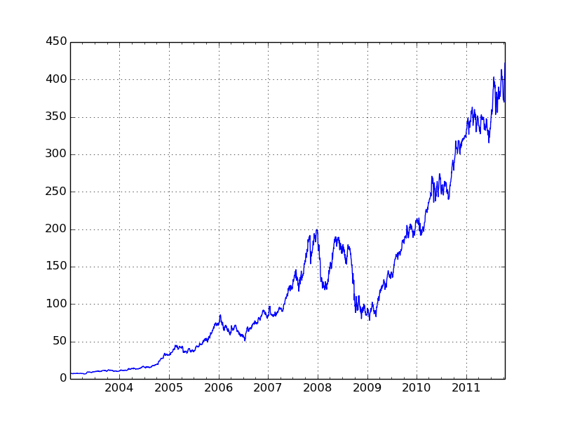
Share Prices
时间序列的绘图
导入几只股票的价格数据
In
[539]: close_px_all = pd.read_csv('ch09/stock_px.csv',
parse_dates=True, index_col=0)
In [540]: close_px = close_px_all[['AAPL',
'MSFT', 'XOM']]
In [541]: close_px = close_px.resample('B',
fill_method='ffill')
In [542]: close_px
Out[542]:
<class 'pandas.core.frame.DataFrame'>
DatetimeIndex: 2292 entries, 2003-01-02 00:00:00
to 2011-10-14 00:00:00
Freq: B
Data columns:
AAPL 2292 non-null values
MSFT 2292 non-null values
XOM 2292 non-null values
dtypes: float64(3) |
对其中任意一列调用plot生成简单图表
| In
[544]: close_px['AAPL'].plot() |
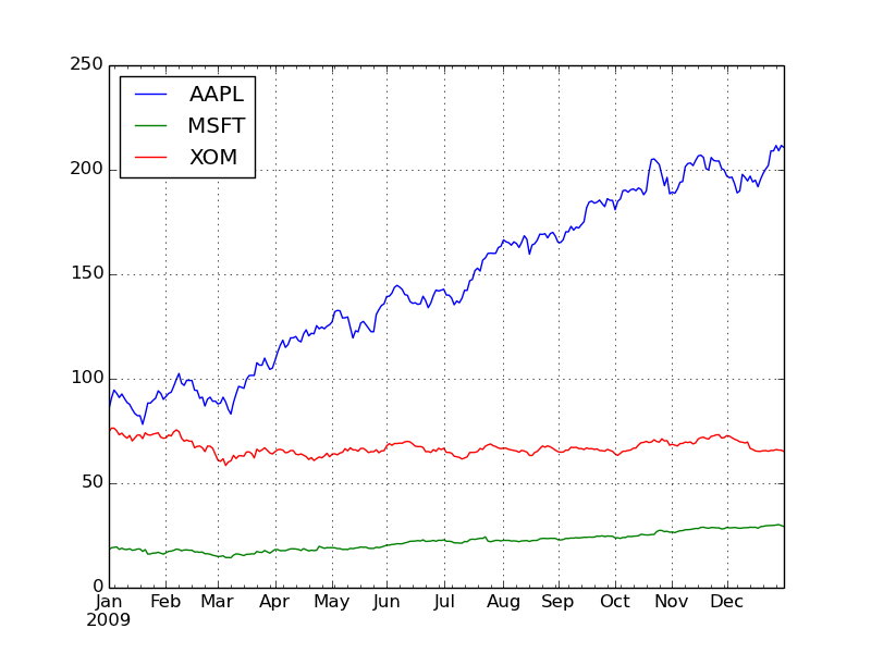
对DataFrame调用plot时,所有时间序列被绘制在一个subplot上
| In
[544]: close_ix['2009'].plot() |
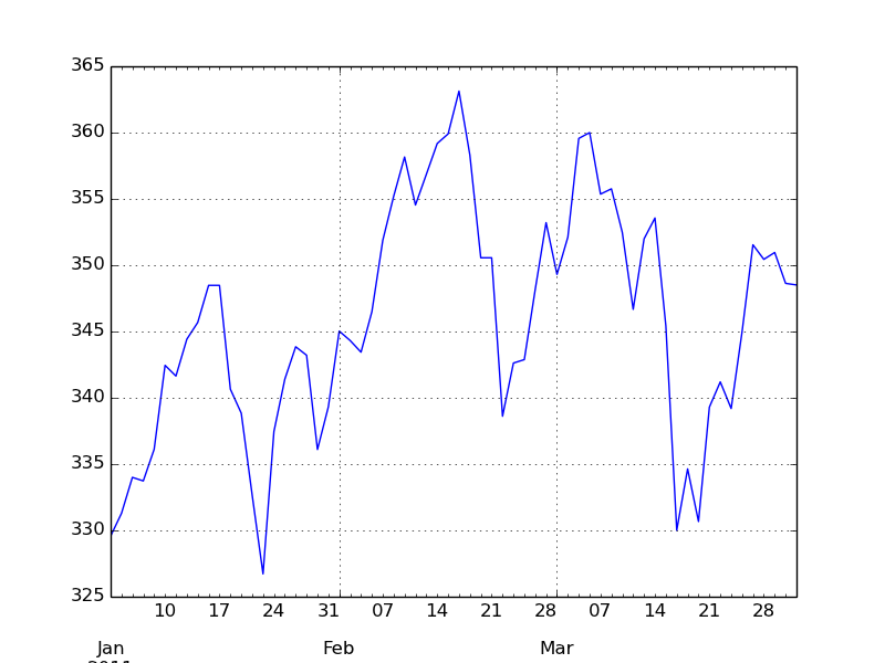
来看看Apple的股价
from January to March
| In
[548]: close_px['AAPL'].ix['01-2011':'03-2011'].plot()
|
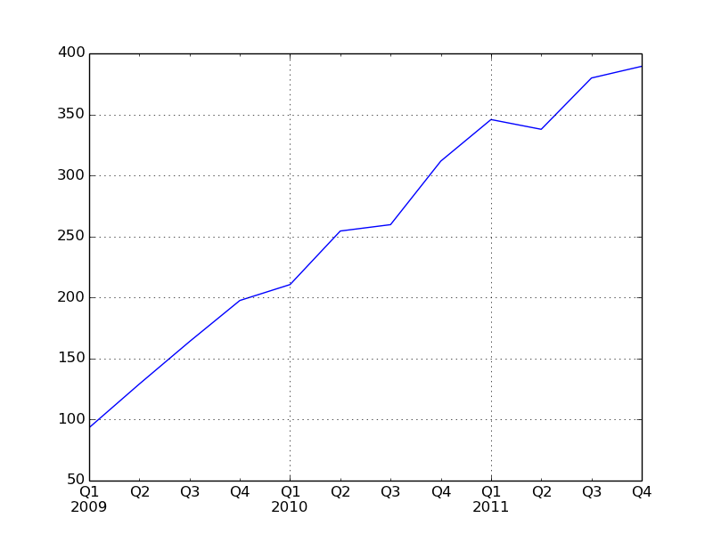
用季度型频率的数据会用季度标识进行格式化
In
[550]: appl_q = close_px['AAPL'].resample('Q-DEC',
fill_method='ffill')
In [551]: appl_q.ix['2009':].plot() |
|